The Nazca Solution

THE RANDOM SIMULATION EXPERIMENT

A Statistical Analysis of the Nazca Great Circle Map-Plateau
By The Nazca Group

To prove that the Nazca Lines represent a great circle map that draws attention to volcanoes, impact craters and ancient monuments, one must design a unique scientific experiment. The goal of the experiment is to test for geographic correlation between the phenomena and the great circles proposed by the Nazca Great Circle Map Hypothesis. To do this one must gauge the correlation between the phenomena and the Nazca great circles and compare it to the correlation between the same phenomena and “random” great circles. By comparing the great circles alignments of the Nazca map with the great circle alignments that result from a randomized version of the map, one can scientifically test the validity of the Nazca Map Hypothesis.
In statistical terminology the random version of the Nazca Map Hypothesis is called the “Null Hypothesis”, and the Nazca Map Hypothesis is called the “Alternative Hypothesis”. The Null hypothesis is the anti-hypothesis that assumes that the Nazca Map Hypothesis is not true. The Null Hypothesis states: “There is no relationship between the sites and the great circles proposed by the Nazca Map Hypothesis. The great circle alignments observed are as likely to occur by random great circle patterns”.
In order for the Nazca Map Hypothesis to be accepted as “true”, the Null Hypothesis must be rejected as “false”. The Null Hypothesis experiment can be said to be the experiment that shows the results of random chance. If the Null Hypothesis experiment results show that the great circle alignments proposed by the Nazca Map Hypothesis are statistically “unlikely” to result from random chance, then Nazca Map Hypothesis must be accepted as true.
Such an experiment that can compare random great circle patterns with those proposed by the Nazca Map Hypothesis can be achieved with a computer program, or computer simulation. The program simulates a virtual Earth with its ancient monuments, volcanoes and impact craters at their exact latitude and longitude locations. The simulation then generates radial centers at random locations on the virtual Earth, with great circles that radiate from them at random angles, or headings.
The Random Simulation program generates a perfectly randomized version of the Nazca Map Hypothesis that can be repeated like any testable and verifiable scientific experiment. The great circle alignments of the random simulation can then be compared with the great circle alignments of the Nazca Map Hypothesis to answer the following question: What is the probability that 79 “randomly” aligned great circles will geographically correlate with as many phenomena as those that result from the Nazca Map Hypothesis?
Before moving on to the Random Simulation experiment some important concepts and terms must be elaborated and defined.

GREAT CIRCLE BANDWIDTH AND SITE DISTRIBUTION

      A great circle alignment is the geographic correlation between specific sites, or locations, and the course of a great circle on the spherical surface of Earth. This geographic correlation is measured and analyzed in reference to the distance of the sites in question to the path of the great circle. If one imagines each great circle as an infinitely thin geometric line encircling Earth, the great circle could be said to encompass, or transect only locations that fall precisely in its path. Due to the large scale and numerous sites involved in the global construct, it would be unreasonable to expect precise linear transections of sites, since the number of phenomena far exceeds the number of great circles proposed by the hypothesis. The Nazca Map Hypothesis claims that each great circle has multiple sites in great circle alignment. The global map construct is of a “Best Fit Line” design similar to the Statistical concept of the “Linear Regression Line” shown in Diagram-1.

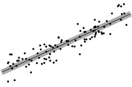
As can be seen in the diagram, several of the points are precisely transected by the thin dark line. Yet the correlation, or association between the line and the other points is evident and the points are said to be scattered about the line. To draw the analogy with the Nazca Map—the “points” are the Site locations of ancient monuments, volcanoes and impact craters and the “line” is analogous to the path of a great circle that circumscribes Earth.

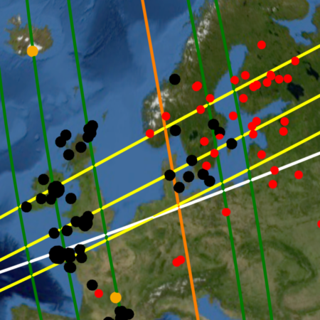
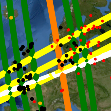
To understand the correlation between the sites and the great circles it becomes useful to visualize each great circle as a great circle “band” having width, or bandwidth as shown in Diagram-1, which shows many more points being encompassed, or transected by the wider grey line. Each great circle band can likewise be visualized as encompassing multiple sites along its course. An example of great circles encompassing (transecting) more sites as they increase in bandwidth can be seen in the comparison between Image-19 and Image-20, which show the same Nazca great circles projected at a different width.

      Any comparison of great circle correlation becomes self limiting at the opposite extremes of bandwidth. If the test bandwidth is extremely narrow neither random great circles nor those proposed by the Nazca Map Hypothesis will encompass any of the sites, nullifying any comparison of great circle correlation. The finite surface area of Earth sets an upper limit to great circle bandwidth. If the great circle bandwidth is wide enough such that 79 random great circle bands cover the entire terrestrial surface, both the random great circles and those of the Nazca map would encompass all the site locations on Earth nullifying any great circle alignment comparison.
The finite spherical surface of Earth also sets a theoretical limit on the geographic distribution of the sites being tested. This limit is best illustrated by its most extreme example: that of an Earth uniformly and completely covered in sites that are equidistant from each other. In such a case any great circle, regardless of its spatial alignment, will encompass the same number of sites, again nullifying any comparison test between random great circles and those proposed by the map hypothesis. Fortunately, the combined total number and geographic distribution of all the sites tested by the random simulation are not extreme enough to induce this “crowded Earth” effect and  the simulation yields significant comparative results.

SITE CATEGORIES

      The term “site” is used in this work in reference to any location of interest for testing geographic correlation with the great circles of the Nazca map and with random great circles. Three principal categories of sites are tested for great circle alignments with the global construct of the Nazca map: Volcanoes, Impact Craters and Ancient Monuments. The Random Simulation program can perform great circle alignment tests on any of these categories individually or in combination.

Monuments

      The monument category is an amalgam of anomalous and extreme structural sites of great age, magnanimity and/or civilizational import. The Nazca Great Circle Map Hypothesis suggests that the ancient monuments were constructed at specific locations on Earth in order to intentionally generate geographic correlation with the great circles of the map. This implies that the monuments and cradle cities were purposefully placed in order to cartographically reinforce the great circles of the map, and draw attention to the volcanoes and impact craters. The global construct of monuments is therefore a cartographic element of the Nazca Great Circle Map; a map whose primary subject is the natural phenomena of Earth.
Many of the monumental sites in the Nazca global construct are part of large structural complexes that were often ancient centers, or cradles, of civilization. The geographic placement of ancient monuments and cities is somewhat locally limited by the terrain and structural needs of each construction – such as stable ground foundations for extremely heavy monuments, the proximity of water sources for cradle cities and other geographic considerations. The global scale of the great circle construct allows for monuments and cradle cities to be placed at cartographic locations that nonetheless reinforce the great circles of the Nazca map. The monumental category can be further divided into sub-categories: monuments, geoglyphic monuments and submerged monuments. The geoglyphic category consists of “graphical” constructs that are either carved into, or formed from the terrain. Nazca, being the most monumental geoglyphic site on Earth as well as the blueprint of the global construct, is categorized as a monument in this work.
The submerged monuments category consists of a growing list of intriguing undersea structures representing the remains of past civilization. Unlike the land monuments, which were geographically placed to reinforce the map; the submerged monuments, like the volcanoes and the impact craters, were the intentional targets of the original great circle alignment.
An additional category of sites called “Other”, contains certain structural and natural phenomena and locations of mytho-historical interest. Some are archeological sites suspected to be locations mentioned in ancient mythology, others are natural phenomena that are central to a particular mythology – such as Mt. Olympus, or Uluru.

Volcanoes

      The term “volcano” is a very broad categorization requiring finer definition. If one were to consider every lava vent on Earth to be a volcano, these would be so numerous and broad in geographic distribution as to induce the crowded Earth effect previously mentioned, nullifying the test. It is logical to expect that the mapmakers would intend to draw attention to the more anomalous and extreme volcanoes of great eruptive power and global climatic significance.
Establishing the eruptive power and catastrophic potential of a volcano is a complex matter. In some cases the eruptive power has been calculated from the remnant signs of past eruptions. The true measure of the eruptive power and potential global climatic effect of a volcano involves the volume, viscosity and chemical composition of the lava in its magma chamber. The general correlation between the volume of the magma chamber and the volume of the mountain-volcano itself, makes volume an ideal attribute for determining the volcano population to be tested. Yet the current scarcity of volcanic volumetric databases leaves “height” as the only practical attribute by which to estimate volume and define the test population for the experiment. The height of a mountain or volcano can be measured in two ways: topographic elevation and topographic prominence. The peak elevation of a mountain is its altitude above sea level, while its peak prominence is its height as measured from its base. A relatively small volcano rising from the top of a high continental massif may present a high elevation from sea level, yet have little eruptive power and global consequence. Peak prominence is the therefore a better indicator of the volume and power of a volcano, and is therefore chosen as the inclusion parameter for the great circle alignment test. The established geophysical category known as “Ultra-Prominent” constitutes volcanoes with peak prominences exceeding 1500 meters. The Ultra category of volcanoes is a clear, established and well defined geophysical category—a suitable and defined population for statistical testing.
An additional subcategory of volcanoes included in the experiment data set are the 16 volcanoes called “Decade Volcanoes”, by the International Association of Volcanology and Chemistry of the Earths’s Interior (IAVCEI). This list is comprised of volcanoes known to be regularly destructive or of particular scientific interest. It is worthy of note that many of these Decade Volcanoes are also Ultra volcanoes.
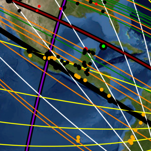
Volcanoes are indeed categorically different from monuments and cities—Nature alone determines their geographic locations. Yet these natural phenomena are not necessarily found in a “random” geographic distribution and under careful inspection certain geographic patterns become readily apparent. Mountain ranges are often associated with tectonic plate boundaries and exhibit the same linear tendency in their geography. It is along these plate boundaries and mountain chains that the majority of the Earth’s volcanoes are found. The linear geography inherent to mountain ranges results in volcanic belts: linear chains of volcanoes that allow for a single great circle to encompass multiple volcanoes. An example of such a volcanic belt is seen in Image-21, showing the Antipodal Orient great circle (black) encompassing beneath its course the linear belt of volcanoes (gold dots) that ridge the Central American Isthmuth. The mapmakers made use of the natural linear tendency in volcanic geography to align the great circles of the Nazca map and thus draw maximum attention to these natural phenomena.

Impact Craters

      Impact craters are the remnant lithospheric scars of cometary or meteoric impacts. The 189 (at the time of writing) currently accepted impact craters accepted in the field of Geophysics provides a well defined and established population for experimental testing. The general correlation between impact crater diameter and impact force allows for selection of crater populations of varying diameter, representing different levels of planetary climatic effect and significance.
Impact Craters present a more random geographic distribution than volcanoes. Their scattered random distribution is intermittently interrupted by crater “clusters” in certain regions of Earth. An example of such a cluster is seen (red dots) in the densely cratered region of northern Europe around Scandinavia, shown previously in Image-19 and Image-20, or the densely cratered continent of Australia seen in Image-16 of the hypothesis section (Part 1). The Nazca great circles seen transecting the crater cluster exemplify how great circles can be aligned to encompass multiple impact craters beneath their courses, enhancing the best fit pattern and drawing attention to these phenomena.
Volcanoes and impact craters abide by other geographic patterns that are implied by the Nazca map and the global construct it illustrates. These geographic patterns suggest great geophysical import and will be addressed in a following section, after the Random Simulation puts the Nazca Great Circle Map Hypothesis through its scientific test.

THE RANDOM SIMULATION

The Random Simulation is a JavaScript computer program that runs on any modern Web Browser. The Random Simulation uses two main data sets to perform its calculations: the Great Circle Data Set and the Site Data Set.

The Great Circle Set

Once the program is active it displays a series of boxes as seen in Picture-6. The box titled “Nazca Parameters” lists the latitude and longitudes of the five Nazca Radial Centers (RCs) and the number of great circles (CGs) that radiate from each. These parameters represent the data of the Nazca great circle map which are provided in Table-8 in the Data section along with the angles of each line on the plateau relative to its anchoring primary line and the true headings of their corresponding great circles. The Nazca parameters are a part of the simulation program and are not user alterable.

The small box titled “Settings” contains the input parameters the user can interactively change. The first input box titled “number of runs”, is the number of times the random version of the great circle map is to be simulated in the trial. Each run represents one cast of 79 randomized great circles. The default is set at 10,000 runs per trial. The higher this number off runs in an experimental trial, the longer the experiment run time, but the more statistically accurate the results yielded.
In each run the simulation generates four radial centers at random coordinates on the virtual Earth, with a fifth radial center at the antipode of one of these. The simulation then generates 79 great circles that radiate from these five radial centers at random angles, or headings. Each “run” thus represents one “random instance”, or random version of the great circles pattern of the Nazca map. The results of each trial forms a Bell Curve for statistical comparison of the pattern of chance with the pattern of the Nazca map. The greater the number of runs simulated per trial, the more complete the Bell Curve that forms from the results. From the Bell Curve produced by the results one can calculate the statistical probability of “random chance” resulting in great circle alignments comparable to those of the Nazca map. The greater the number of runs in a trial, the more statistically confident one can be in the calculated probability of random occurrence.
The input parameter, “Bandwidth” is the width of each great circle band in kilometers. This bandwidth applies to both the Nazca great circles and their random counterparts. If one inputs a 20 kilometer bandwidth the simulation will make each of the 79 Nazca great circles into bands 20 kilometers in width, and count the number of sites they encompass. The simulation then assigns the same 20 kilometer width to each great circle in the randomly generated sets of 79 and counts the number of sites encompass in each random iteration.

The Site Set

The large scrollable box labeled “Sites”, lists the monuments, volcanoes and impact craters available for the random simulation test and their latitude and longitude coordinates. Each site has a check box for individual inclusion or exclusion from the test. The sites appear on the list in order by category.
Ancient monuments and cities are listed first in alphabetical order. This list of ancient monuments and their coordinates is also provided in Table-5 in the Data section. There are several subtypes of monuments that are grouped together under categorical labels such as, “Pyramid”, “Menhir” or “Dolmen” in order to facilitate locating them on the list. There are exceptions to this grouping such as the Great Pyramid of Giza which is found alphabetically under letter “G” and not with the other pyramids.
The monument names which are written in capital letters represent those that serve as capitals of their monumental groupings. The capital groups are defined by a 50 kilometer radius from the capital monument and between satellite monuments in the group. If a monument is within 50 kilometers of a monument that is within 50 kms of a capital monument, both satellite monuments belong to that capital group. Therefore, if a monument is 50 kms or more from a capital monument or any of its satellites, it does not belong to any group and is considered a lone monumental site. All the monuments that are in the immediate vicinity of the Giza Plateau, for example, are part of the “Giza” group. This allows one to select the Great Pyramid as the single representative of the entire Giza group that would otherwise include the other many pyramids and monuments of the Nile Delta region. One can thus test entire groups or only the “Capital” monument of each group. The capital of a monumental group is, as best determined, the most anomalous or extreme structure of the group, as best determined. At the end of the monuments list is comprised of the subcategories, “Geoglyph”, “Submerged Monuments” and “Other”, followed by the impact craters as seen in Picture-7.

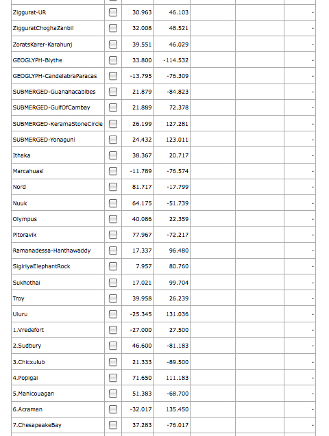
      The currently accepted impact craters are numbered in order according to crater diameter to facilitate selection of test populations in terms of impact force and global climatic effect. The impact craters list with their coordinate locations, diameters, approximate ages and force of impact if available are also provided in Table-7 in Data section.
The volcanoes of Earth comprise the end of the site list and are grouped according to the continental plate on which they are found. Within each continental grouping the volcanoes are roughly in order by decreasing topographic elevation, not according to topographic prominence. The “Ultra” volcanoes with a topographic prominence exceeding 1,500 meters are in their respective continental plate groups in capital lettering for easy identification. The list of volcanoes with their coordinates, topographic elevation, topographic prominence and Volcanic Explosive Indexes (VEIs) is provided in Table-6.

       The box labeled “Selections” allows the user to select and deselect entire categories and subcategories of sites to facilitate management of the list. All monument groups and capitals combined into a group, are available for selection. The impact crater selections constitute divisions at different crater diameter by “tens” of kilometers groupings. The volcanic subcategories “ULTRA” and “DECADE”, as well as by continental plates groupings, all are available as selections to customize the random simulation test.

Results Output

Once the great circle parameters and sites have been set, the random simulation is ready to run. The box labeled “Results” seen in Picture-8 the output boxes for various numerical results and the simulation “Run!” button. The empty window within the box is where the results of each run are outputted. Each number is the total number of “Hits”, or sites encompassed by the 79 random great circles in one simulation run. If the trial consists of 10,000 runs, 10,000 results will be displayed in the scrollable box at completion.

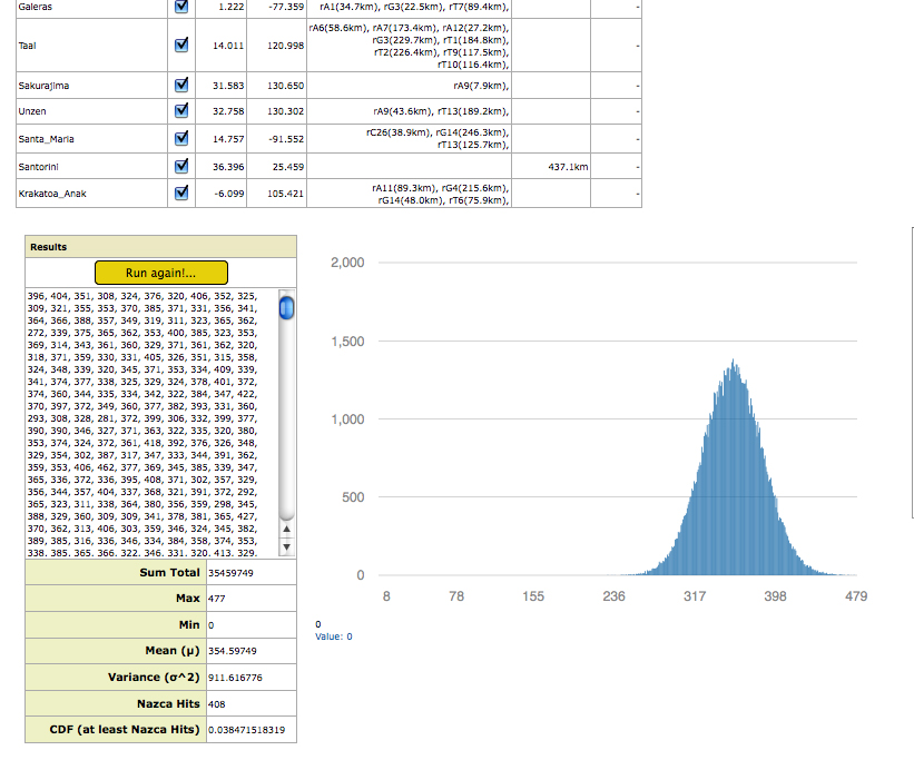
      At completion the program lists which great circle(s) transected each site and at what distance the site is from the great circle(s), as seen in the top left window  in Picture-8. at what distance from the center of the great circle the site is. For sites not transected by any great circle at the tested badwidth, the program lists the distance to the nearest great circle.

      Below the scrollable results box a series of numerical output boxes that  display the results of the following statistical calculations:

Sum Total: The sum of the hits of all run results in the trial.
Mean: The statistical mean, or average of the total number of “Hits” (sites
encompassed) for all run results.

Max:     The maximum number of sites encompassed by a single simulated run in the trial.

Min:     The minimum number of sites encompassed by a single simulated run in the trial. At the great circle bandwidths and number of runs per trial that are adequate for the test the minimum tends to remain zero—at least one cast of random great circles not encompassing any sites thus resulting in zero.

Variance:    The statistical Variance of the results of all runs in that trial. Also known as “Sigma Squared”.

Nazca Hits:   The total number of sites encompassed (transected) by the great circles of the map at the bandwidth being tested.

CDF:   The Cumulative Distribution Function result is the calculated Probability of Random Occurrence, or the probability that random chance has of achieving the same results as the Nazca Great Circle Map Hypothesis at the tested great circle badwidth.

In addition to these numerical results the random simulation graphically displays a Distribution Curve of the results, seen also in Picture-8. The X-Axis of the curve is the discrete number of possible encompassed sites, or “Hits”; the Y-Axis is the total count of random runs that resulted in that number of encompassed sites. The distribution curve displayed is cursor-interactive; numerically displaying the number of runs for each “Hit ” value at the lower left corner of the Distribution Curve window.
As previously mentioned, the Random Simulation yields the results of each trial in a the Results box along with a distribution curve as seen previously in Picture-8, which shows a well defined distribution curve.
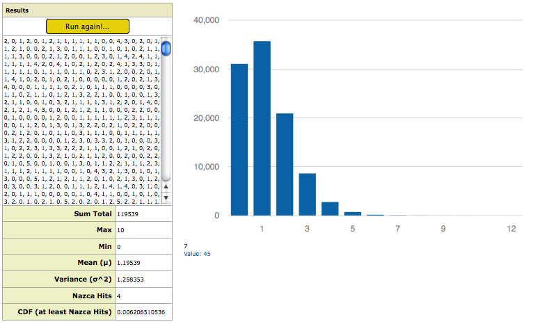
At narrow great circle bandwidths of only a few kilometers, few sites are encompassed and the distribution curve is therefore incomplete, as can be seen in Picture-9, which shows the results and distribution curve from a test trial on all impact craters at 1 kilometer great circle bandwidth. The incomplete “half-bell” shape of the distribution curve is due to the fact that at narrow great circle bandwidths there are many random great circle runs that yield “Zero Hits”—no sites being encompassed, or transected by any of the randomized great circles.

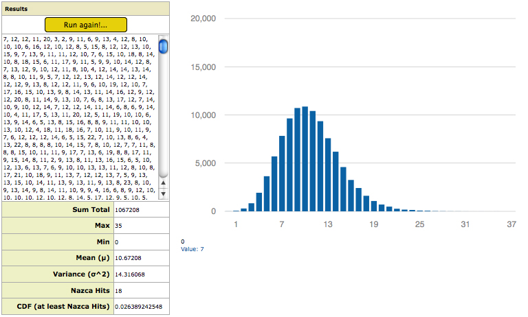
     The Cumulative Distribution Function (CDF) requires a complete distribution curve to accurately calculate the probability of random occurrence. The probability results of the simulation are therefore not valid at very narrow great circle bandwidths. As one increases the width of the great circles the simulation results in less instances of “zero hit” runs and a complete distribution curve begins to form. Picture-10 shows a complete distribution curve begin to form at around 8 kilometers of great circle bandwidth for the impact craters trial. It is at this great circle width, or greater, that one may have statistical confidence in the results for that particular category of sites (all impact craters). The specific bandwidth at which a complete distribution curve forms varies with site category being tested, yet all categories show a clear distribution curve forming at a great circle bandwidth of 8 kilometers.

THE NULL HYPOTHESIS EXPERIMENT

      The Random Simulation provides the experiment and data for the statistically analysis of the Nazca Great Circle Map Hypothesis. The initial experiment entails a complete scan of great circle bandwidth on the following four site categories: 1. Monuments, 2. Volcanoes, 3. Impact Craters, and 4. All three categories combined.
This initial experiment excludes the subcategories of monument sites: submerged sites, geoglyphic sites (with the exception of the Nazca Geoglyphic Monument itself), and the category “OTHER”. These excluded subcategories are available for selection in the simulation for any user to test individually or in combination. A few new monuments have been added to the list since this experiment. These additions only improve the result. The population tested for the experiment were the Capital Monuments of each monument group and those not satellites of a monument group (non-satellite monuments). The volcanoes tested were are all those belonging to the “Ultra” and “Decade” categories. All impact craters accepted in the field of Geology were included in the experiment.
Each experimental trial consisted of 100,000 runs, or 100,000 random map iterations, at each bandwitdth tested. This number of runs was determined, through trial and error, to balance statistical accuracy of the results with computation times. At 100,000 runs per trial there is very little variance in the trial results and these produce well defined Distribution Curves that allow the Cumulative Distribution Function (CDF) to yield accurate calculations of the probability of random occurrence.
In order to reduce computation times each scan begins at 1 kilometer great circle bandwidth, then 5 kms, then 10 kms and increasing by 10 kilometer increments each trial thereon. The 10 kilometer increments allow the scan of the entire range without the thwarting computation times involved in doing all 1 km increments. However, in the attempt to precisely locate the great circle bandwidth at which the exact maximum(s) occurs, several spans of the scans are in 1 kilometer increments. In the future we hope to provide complete 1km resolution for all data—until such a time a user may test the Random Simulation at any missing great circle bandwidth in question, or use it to verify the results of the experimental presented below.

RESULTS ANALYSIS

      The complete results of the Random Simulation scans are provided in Table-1 to Table-4 in the Data section where the experiment results for the monumental, volcanic, impact crater and all categories combined are tabulated. The right side columns of the tables give the probability of random occurrence and can be seen to vary with both great circle bandwidth and between site category—each category peaking in probability by different amounts and at different great circle bandwidths.
In statistical analysis, “statistical significance” is the point at which the probability of an event occurring randomly is considered to be sufficiently unlikely to reject the Null Hypothesis and accept the Alternative Hypothesis. This significance level is often set at .05 (5%) or .01 (1%). This is to mean: If random chance reproduces the effect less than once in twenty, or less than once in one hundred times, the Alternative Hypothesis (Nazca Map Hypothesis), must be statistically accepted as true.
The probability of occurrence of great circle alignments shown by this experiment is far above the threshold acceptance level for each category of sites, within a broad range of great circle bandwidths.
To help visualize the data, graphs of the probability of random occurrence according to great circle bandwidth for monuments, volcanoes, impact craters and all three categories combined, are presented below.

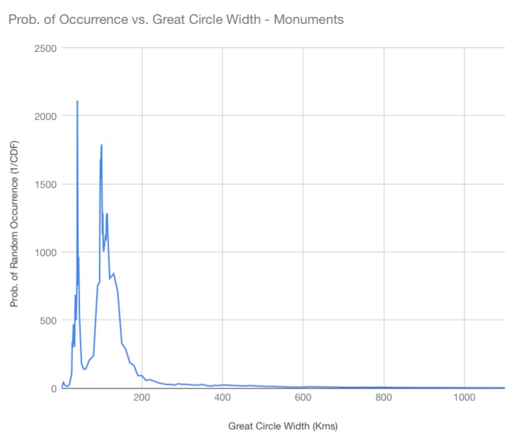
The horizontal axis of the graphs represent great circle bandwidth in kilometers. Since the Continuous Distribution Function (CDF) yields results as decimals, the graph plots 1 / CDF, to represent the Probability of Random Occurrence and avoid graphing a decimal on the Y-axis. The higher the probability peak on the Y-axis of the graph, the less likely that the Nazca great circle alignments could be the result of random chance for great circles of that bandwidth.
The first graph for the ancient monument category shows a peak at 40 kilometers great circle width with a probability of random occurrence of 2112—the random great circles only achieving geographic correlation with monuments, equivalent to the Nazca map’s great circle alignments, only once in 2112 random iterations. This is 100 times greater than required for statistically significance. The strength of correlation is evidence of the monuments being in purposeful great circle alignment with great circles of the Nazca map.
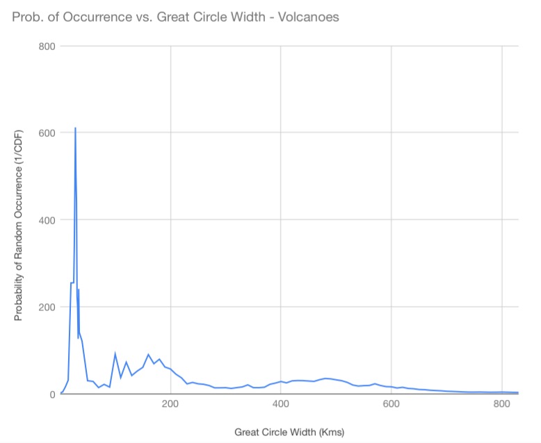
The second graph shows the result for the volcanic category. The peak occurs at 28 kilometers great circle bandwidth, with a probability of random occurrence of once in 612 random iterations; 6 times greater than required for statistical significance.
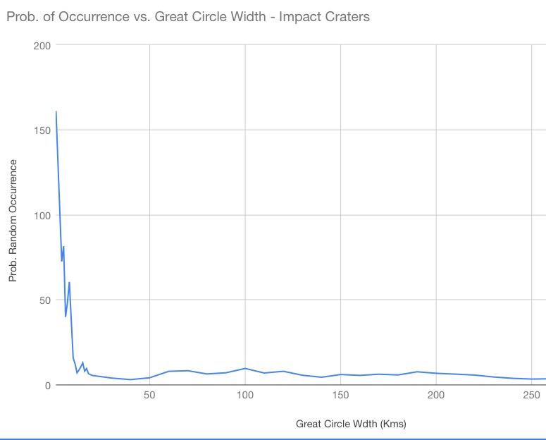
The last graph shows the results for the impact crater category. The peak occurs at 1 kilometer greats circle width and a probability of random occurrence of once in 161 random iterations. As previously mentioned, however, the distribution curve is incomplete until about 8 kilometers of great circle width. We therefore consider 8 kilometer great circle width to be the start of statistical confidence. The maximum is therefore at 9 kilometers great circle width and probability of random occurrence of once in 37 random iterations. This is still nearly twice the generally accepted, ” once in 20 “, minimum threshold. This is clear evidence of correlation with the great circles of the Nazca map, but not as strong as the other two categories. The lack of both natural and artificial linearity in the geographic distribution of impact craters—their geographic randomness—is the likely explanation. Volcanoes, having more geologic linearity, are more easily incorporated into great circle alignments, snd the monuments are purposefully placed in order to reinforce the the great circle alignments.
The last graph shows the results for the monuments, volcanoes and impact craters combined category. At a great circle bandwidth of 29 kilometers the probability of random occurrence is once in 42,028 random iterations…. 420 times the required statistical threshold.
The fact that all categories combined reaches a probability of random occurrence far greater than any individual category constitutes overwhelming evidence that all the categories have great circle alignment with the great circles of the Nazca Map.
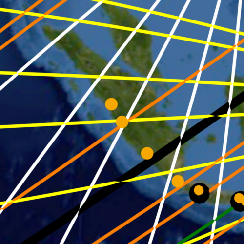
This initial experiment does not take into account triangulation or hierarchy. In other words, it does not test for the fact that in many cases the larger volcanoes and impact craters are “triangulated”, or transected, by more than one great circle. An example of this prioritizing can be seen in Image-21, where the third largest known meteor crater (red dot) Chicxulub – nemesis of the dinosaurs – is triangulated by two Nazca map great circles at the tip of the Yucatan Peninsula. A volcanic example of the same principle is seen in Image-22, showing the triple great circle transection of Mount Kerinci—largest volcano in Sumatra and one of the largest on Earth. Random simulation tests that include multiple transections upon single sites will be run and added to this work in the near future.
It is worth noting that the ancient monuments for testing by the random simulation experiment are a broad population in an attempt at being inclusive and non biased. In other words, the list of monuments gives the Null Hypothesis the advantage. It is a fact that if one selected only the sites known to be encompassed by the Nazca great circles the experiment would retain scientific and statistical validity—the Random Simulation would still calculate an accurate probability of occurrence of even greater statistical significance.

CONCLUSION

The Nazca Great Circle Map Hypothesis, as tested by the Random Simulation program, yields overwhelming statistical evidence of being true. The geographic correlation of ancient monuments, volcanoes and impact craters with the great circles of the Nazca map is statistically unarguable.

The empirical evidence in the form of newly discovered accepted impact craters and ancient monuments will continue to strengthen the proof presented here. In fact, we encourage all people to use the Nazca great circle map to assist in the rediscovery of our past, and all that remains hidden in Earth majesty.

By Frank Maglione Nicholson (statistical analysis, testing and graphics) and David Grimason (programming, statistical analysis and testing ), with thanks to Ken Phungrasamee (testing and graphics).

© 2020